
TLDR:
Learned proximal networks (LPN) are deep neural networks that exactly parameterize proximal
operators.
When trained with our proposed proximal matching loss, they learn expressive and interpretable priors
for real-world data distributions
and enable convergent plug-and-play reconstruction in general inverse problems!
We propose learned proximal networks (LPN), a class of neural networks that exactly implement proximal operators of general (possibly nonconvex) functions, and a new training loss, dubbed proximal matching, that provably promotes learning of the proximal of an unknown prior.
LPN achieves state-of-the-art performance for inverse problems, while enabling precise characterization of the learned prior, as well as convergence guarantees for the Plug-and-Play algorithm.
We study the prior learned via training with the proximal matching loss versus other common denoising losses, such as $\ell_2$ or $\ell_1$ loss.
In a toy setting where we know the true prior, we see that LPN with proximal matching learns the correct proximal operator, while other losses do not!

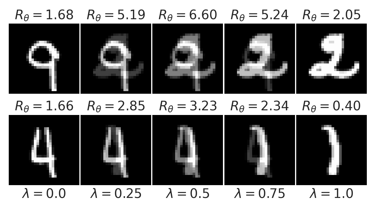
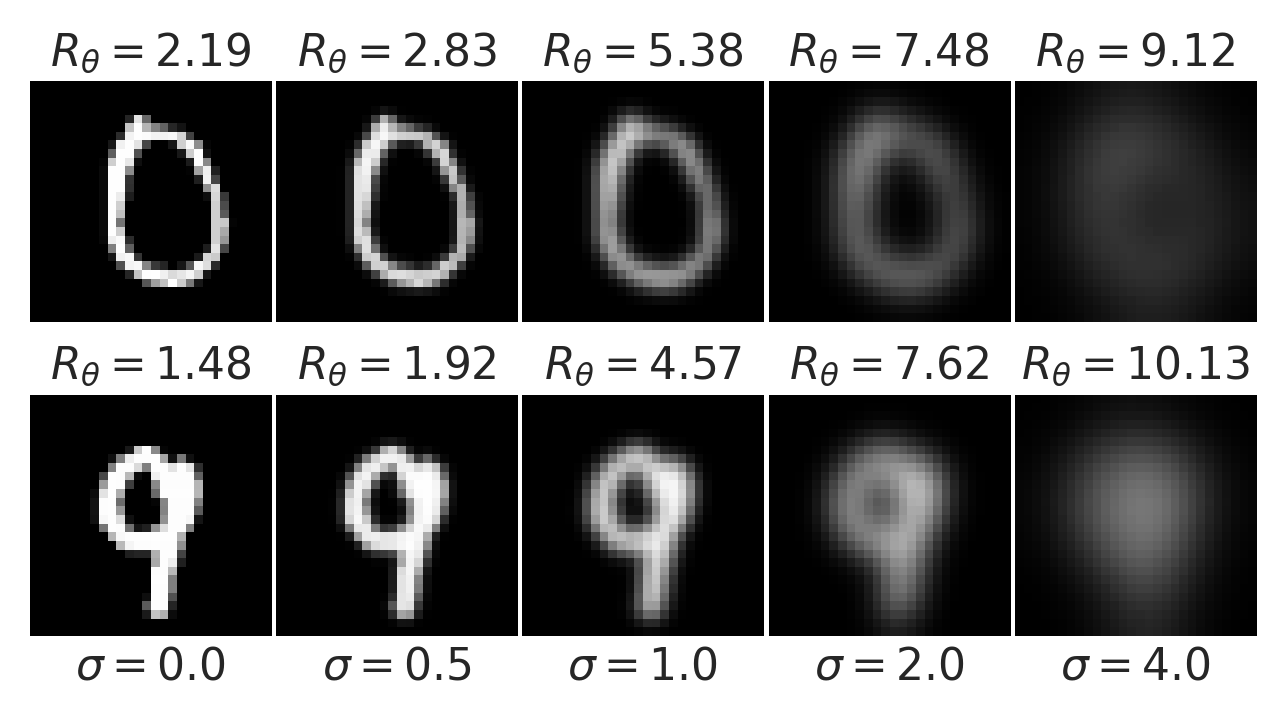
The implicitly-learned LPN prior faithfully captures the distribution of natural hand-written digit images.
The learned prior, $R_\theta$, evaluated at images corrupted by additive Gaussian noise with standard deviation $\sigma$:

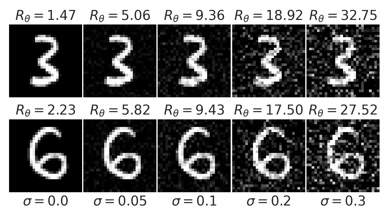
The learned prior, $R_\theta$, evaluated at the convex combination of two MNIST images $(1-\lambda)\mathbf{x} + \lambda \mathbf{x}'$, showing that the prior faithfully captures the nonconvex nature of natural image data distributions:

The learned prior, $R_\theta$, evaluated at images blurred by Gaussian kernel with standard deviation $\sigma$:

CelebA deblurring for Gaussian blur kernel with standard deviation 1.0 and noise level 0.02:
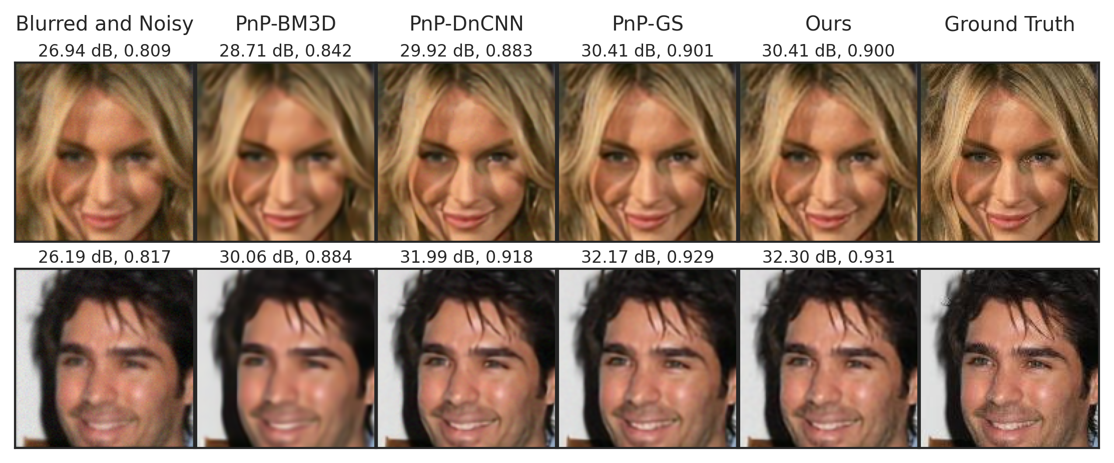
Deblurring with blur kernel standard deviation 1.0 and noise level 0.04:

Sparse-view tomography (undersampling rate $\approx$ 30%):

Compressed sensing (compression rate = 1/16):

Additional experimental results and all experimental details are available in the paper.
We make use of a mathematical characterization of proximal operators due to Gribonval and Nikolova, which states that a map $f$ (with sufficient regularity) is a proximal operator if and only if it is the gradient of a convex function (with corresponding regularity). The following diagram illustrates these relationships for the $\ell_1$ regularizer.

This extends Moreau's classical characterization of proximal operators of convex functions, giving us a basis for learning proximal operators for general, nonconvex regularizers! LPN applies the input-convex neural network architecture of Amos, Xu, and Kolter to obtain an exact parameterization of (continuous) proximal operators.
Gribonval (2011) pointed out that MMSE denoising under the classical Gaussian noise model $$ \boldsymbol{y} = \boldsymbol{x} + \boldsymbol{g}, $$ where $\boldsymbol{x} \in \mathbb{R}^n$ is distributed according to a prior distribution $p$ and $\boldsymbol{g}$ is independent isotropic Gaussian noise, does not correspond to penalized MAP estimation with the log-prior $-\log p$. In other words, learning a deep denoiser via minimum $\ell_2$ denoising does not recover the correct log-prior for the underlying data distribution!
To overcome this limitation, we propose the proximal matching loss for learning expressive priors. It writes $$\newcommand\x{\boldsymbol{x}}\newcommand\y{\boldsymbol{y}}\newcommand\E{\mathbb{E}} \mathcal L_{\gamma}(\x,\y) = 1 - \frac{1}{(\pi\gamma^2)^{n/2}}\exp\left(-\frac{\|\x-\y\|_2^2}{\gamma^2}\right), \quad\gamma > 0. $$ In contrast to MMSE denoising, we prove that in the limit of small scale parameter $\gamma$, training a denoiser by minimizing the proximal matching loss recovers the correct log-prior!
Suppose we have linear measurements $\boldsymbol{y} = \boldsymbol{A} \boldsymbol{x}_{\natural}$ of a high-dimensional vector that we wish to reconstruct. With a prior $p$ for $\boldsymbol{x}_{\natural}$ that we can evaluate, we can do this by solving the regularized reconstruction problem $$ \min_{\boldsymbol{x}} \frac{1}{2}\left\| \boldsymbol{y} - \boldsymbol{A} \boldsymbol{x} \right\|_2^2 - \lambda \log p(\boldsymbol{x}) $$ with solvers from numerical optimization (e.g., proximal gradient descent or ADMM). Such solvers involve the proximal operator $\mathrm{prox}_{-\lambda \log p}$ for the log-prior.
If we want to avoid modeling the distribution $p$ by hand, we can replace all instances of this proximal operator with a pretrained deep denoiser $f_{\theta}$. This corresponds to a plug-and-play (PnP) reconstruction algorithm for the underlying inverse problem. This motivates a natural question: when can we guarantee that a PnP scheme converges?
A priori, replacing a proximal operator with a general deep denoiser takes the PnP iteration outside of the purview of convergence analyses from numerical optimization. However, because LPN exactly parameterize proximal operators, we obtain convergence guarantees for PnP schemes with LPNs for free under essentially no assumptions. We provide proofs of such convergence guarantees in our paper, for PnP-PGD and PnP-ADMM.
This material is based upon work supported by NIH Grant P41EB031771, the Toffler Charitable Trust, and the Distinguished Graduate Student Fellows program of the Kavli Neuroscience Discovery Institute.
This website template was adapted from Brent Yi's project page for TILTED.